
Boris.T.Fedosov
Rudny Industrial Institute,
Rudny, Kazakhstan
About author
UDC 681.51.01
F338
The student should have possibility to obtain
the information in the accessible form
if he has abilities, due preparation and desire
to master a subject.
Real industrial objectss of control usually are multi-dimensional, i.e. have some inputs and some outputs. In some cases such objects can be modelled, neglecting the minor actions, and also the minor controlled variables. As a result of such justified simplification it is possible to gain a simple model with two (operating and disturbing), and in some cases and with one action, and with one controlled variable. It essentially simplifies both the object analysis, and development of automatic control system of it.
However in many cases it is necessary to ensure control of several controlled variables of the object, its output variables, by action on some its inputs, i.e. modifications of controlling variables, plus to that should be considered also some disturbances. The control singularity such, difficult enough object in exposition, consists that can happen that action on one entry leads to a modification not to one, and at once several controlled variables. For example, on some estimates [7-2], in chemical processes of the order of 15 % make doubly linked control systems. We will illustrate singularities of multi-dimensional objects of control with following instances.
Let there is a car. If it goes, and the driver slightly will turn a steering wheel on the left also the car will start to turn to the left. If the driver adds to gas the car will go faster. It is obvious. We will imagine the envisioned car which at rotational displacement of a steering wheel not only turns, veers motions, but also it is sped up. Having such car, the holder a bad word will remember its manufacturers, but, not having another, will be compelled to be accustomed to that is. To turn the car it is necessary not only control steering wheel displacement, but also simultaneous decrease of gas if it is required to turn on the same velocity. Eventually, and it is possible to be accustomed to it.
Certainly, nobody will producted such envisioned car, as nobody will buy it. But here with helicopters absolutely an another matter. They behave so, and, nevertheless, them use. Really, if the pilot of the helicopter wishes to be sped up, it, naturally increases gas submission. However only it does not lead to velocity magnification: the rotor starts to be spun faster, and the helicopter is aimed to mount. Moreover, a speed-up of twirl of a rotor forces the helicopter also to be turned round an axis of yaw, reversing direction driving. So, to speed up helicopter flight at the same altitude and in the same direction, the pilot should increase fuel supply and simultaneously increase thrust of an aft propeller, changing an angle of attack of its lobes and also to incline the helicopter forwards (more precisely to warp a plane of twirl of lobes of a principal propeller) that added by magnification of gas power was outlayed for flight forwards a little. To it to operate helicopter where is more difficult, than an airplane for which controlled variables if are interdependent where to a lesser degree.
Thus, there are the objects which controlled variables depend on several control both disturbing actions and control of such objects difficult enough occupation.
For the description and examination, stabilising and optimisation of multivariable systems the solid mathematical apparatus [1], in particular decomposition techniques and decentralisings, Lyapunov's vector functions, etc. This apparatus on the one hand uses, the high mathematical culture, but with another demands enough, in view of the generality, essentially hampers understanding of engineering, physical essence of control procedure. Job on the analysis and optimisation of control system is reduced to execution of some mathematical operations in which outcome the control system can be gained optimum somewhat. However it is rather useful for development engineer to feel properties of designed and researched system, that it is qualitative (in sense not quantitatively) to inspect optimisation process
The present article purposes evident consideration of singularities of description of multi-dimensional objects and control of them, allowing to achieve understanding of an essence of case.
Distinctive singularity of real multi-dimensional multivariable objects is that every output, the controlled variable depends not on one, and from several input, controlling variables, and also several disturbances. As is shown in the instances resulted above, in introduction, control of such object can appear difficult task.
For simplification of control by multi-dimensional objects try to "disentangle" output variables so that every output, the controlled variable depended only on own operating input. But even at implementation of such decoupling at the subsequent actuation of the multi-dimensional object in control loops, it appears, that in a control system originate more or less difficult of an outline which, basically, potentially can lead to loss of stability by a control system. Losses of stability also need to be avoided at control system design.
The dinamic regime of operation of the object implies, that actions on it vary in time that leads to exhibiting of inertia-oscillating properties of the object, and also to exhibiting of the delays available in him linked to distribution of signals.
Let's observe some object two-input-port and two outputs. On the first input we will give a unit step, and after a while we will give a step and on the second input:

Fig. 1.1.1.1. On the oscillogram the first output variable as time function is displayed only not to overcharge the plot. The first output variable depends not only on action on the first input, but also from action on the second input
By an initial part of the oscillogram of the first output variable y1 it is possible to draw a conclusion, that the first forward channel u1 → y1 represents a series connection of an aperiodic link of the first order having time constant, equal about 0.3 sec, and a delay link on 1.5 seconds. On the eighth second there is a stepwise unit step input on the second input of the object, and it leads to the decrease of the first output variable having damping oscillating character. Frequency and a velocity of damped vibrations, and also the gain of the first output variable called graduated modification by the second control signal, allow to size up parametres of the oscillating link linking the second input with the first output.
Thus, at control of the multi-dimensional multivariable object it is necessary to consider and compensate response of controlled variables to others, except "own", control action, which can be observed from the point of view of control of the object on the first controlled variable as disturbances
Let's look, that is in the composite unit of the linear model of 2D-object of control:
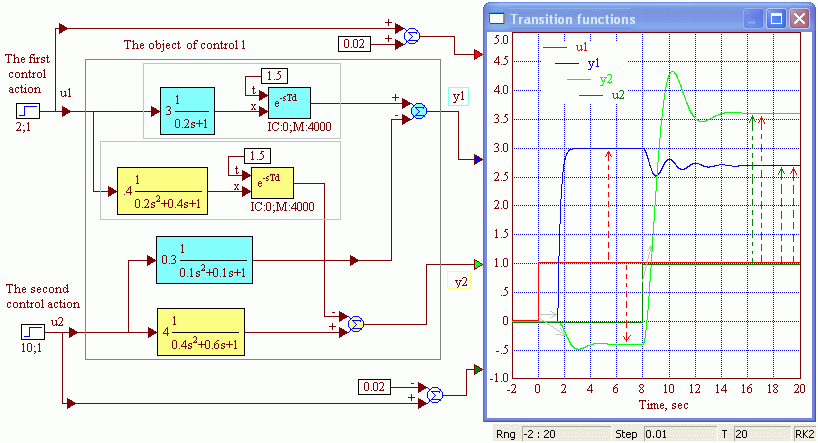
Fig. 1.1.1.2. The structure of the observed object displays, that links are available from each input to each output. Apparently, each output variable depends not only on an own controlling variable, but also from other variable which can be observed as disturbance. Essentially in real linear objects of link can be more difficult, but them it is possible to lead approximately to such kind unless delay links can appear also in other links
The description a method "Input - Output" links output signals of model to each input. In the field of Laplace image such description is implemented by means of transfer functions on each link:
(1.1.1.1)
![]()
or, in a matrix form:
(1.1.1.2)

Advantage of the description on a method «Input - Output» consists that it is possible to trace in an explicit form signal passage on all branches of model from any input to any output. Disadvantage of the description that at major number of input and output variables operation under the analysis of properties of system becomes rather labour-consuming.
The static operation regime of system or object of control this is their functioning at stationary values or rather rather slowly varying input actions when transient phenomena or were already completed, or they give negligiblely small contribution in comparison with current meanings of output's, controlled variables. Essentially, as a rule, the bulk of an operating time of standard industrial plants transits in a regime of a statics or close to it a regime that determines its significance by consideration of properties of the object.
The linear static model of control object is good that is evident and consequently in view of the obviousness widely uses in practice. Really, practically any mechanic, both by itself the master and the operator serving some technological object, will easily answer on a question, on this or that controlled variable how much will mount or will be reduced if slightly to increase the controlling variable or disturbance.
The linearized multi-dimensional object of control can be presented in a static regime by a matrix with fixed coefficients [16, 17]. The equations follow from (1.1.1.2) at substitution р = 0 and passage in time domain, in field of originals.
For example, for the object having two input actions and two controlled variables, static model looks like this:
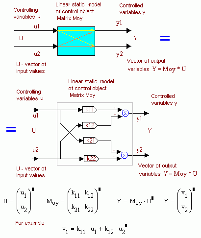
Fig. 1.1.2.1. The description and control of the object in a statics regime
The sense of coefficients of a matrix Moy, characterising of the object operation a static regime, is obvious and clear. These are gains of signals on the appropriate channels displayed by arrows. These coefficients have generally different physical dimensions of a quantity. Physical dimensions of a quantity of coefficients is determined by dimensions of a quantity of input and output variables of the object of control.
Generally the linear object every output, the controlled variable is determined by all controlling variables, representing their weighed total.
It is known, that practically all real objects and systems are nonlinear and continuous. Method «Input - Output» limitation consists in usage of the linear model. But infinitesimal changes of actions on the nonlinear object lead to small, proportional modifications of its responses. Simulation of objects at enough infinitesimal changes of actions allows to present their simple equations, in particular on a method «Input - Output». And linearity of model essentially simplifies the analysis of control systems by their operation in regimes, close to nominal, close to a point in which the object model linearization is conducted.
The complete description of nonlinear model of the multi-dimensional object willy-nilly should be executed a state-variable approach.
The alternative simulation method of nonlinear multi-dimensional objects and systems this numerical object-oriented simulation in special programs, for example in program Vissim.
The state-variable method uses for the description of multi-dimensional objects and systems. Its application is stipulated by that the equations of various objects have a standard appearance that allows to parse their properties, in particular stability, by standard methods.
The differential equations presenting the dynamic object of control, it is possible to lead to a set of equations of the first order of a standard kind, i.e. to present them in the so-called form of Cauchy. Variable set of equationses are called as state variables. If each subsequent state variable is a derivative on time from previous such variables are called as the phase variables.
For linear objects without links of delay the equation in state variables look like [2]:
(1.2.1.1)

Thus, the set of equations (1.2.1.1) links a gang, a vector of output variable {yk} to a gang of input actions {ui} via "interior" state variables {xj} the multi-dimensional object. At first sight, introduction of "intermediate link" what the gang of state variables is, complicates the system definition. However it not so. Along with that the description (1.2.1.1) has a standard appearance that essentially simplifies, does einartig the analysis and the solution of the equations presenting the object, such description gives also a certain methodological sight at the linear object. Really, the equation
(1.2.1.1,a)
![]()
in state variables taking into account initial conditions, i.e. values of state variables in a conditional zero time moment, completely, comprehensively presents owns, absolute properties and behaviour of the inertial object at absence of external actions.
Let's mark, that the matrix A contains exactly the same information on absolute, own properties of the linear object, as its characteristic polynomial, in particular, informations about a degree of stability of the object. To this object, by means of a matrix B the gang of external actions matching to a real situation necessary to the researcher can be applied. And, besides, by means of a matrix C it is possible to set, determine, as output variables depend on state variables, ensuring correspondence to the modelled real object.
Let's mark, that in the literature uses also other purposes of matrix D, but matrixes A, B and C use only how in (1.2.1.1). The equations (1.2.1.1) concerning matrix D are recorded here so because in such kind they use in Vissim’е in which their matrixes of known, preset structural model will be determined more low .
Writing of equations of state in the form of (1.2.1.1) leads to the standard form of the block diagramme of an object model:
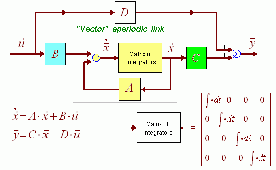
Fig. 1.2.1.1. The structural vector model of the linear multi-dimensional object presented by state variables. The central part of model is multi-dimensional analogue of model of an aperiodic link of the first order. The matrix of integrators of system of the fourth order is resulted for an instance. We will mark, that in the matrix of scheme are multiplied by input vector signals, rather the reverse, as multiplication of matrixes and vectors is noncommutative. The aperiodic link here is named "vector" because its input and output variables are vectors in space of state variables
For the object with two inputs and two outputs the equation (1.2.1.1) can to look like, for example:
(1.2.1.2)
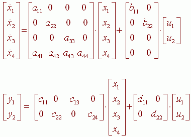
Writing of the equations of state variables of some model, and its subsequent manual analysis is enough labour-consuming and boring operation, that, was possiblly, forces to turn away from this method of engineers-experts. However up-to-date programs of object-oriented simulation (Vissim) allow to automize process of writing of the equations of statuses for the objects builted by structural simulation, and programs of numerically-analytical simulation (Mathcad) allow to perform easily algebraic operations over matrixes and vectors, simplifying the analysis of particular system or the object.
The analysis of properties of model with the preset, known structure and determination of matrixes of its state equations can be executed in Vissim’е, according to standard algorithm [3]. However, on an operation procedure it is required to make some explanations, differently at its mastering there are difficulties.
For determination of coefficients of matrixes of some fragment or the complete object model in Vissim it is necessary to launch simulation and to select an interesting multi-dimensional fragment of the scheme. To click on "Select Input/Output Points" from the list which is falling out at click on menu Analyze, and then clicks to select one input and one output:
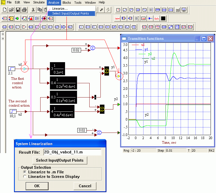
Fig. 1.2.1.2. Determination of coefficients of matrixes of state variables of the selected fragment of model in Vissim and their saving in a file. The first input and the first output of model of the 2D-object are selected, their colour has varied
After input and output selection to click on a spare space on a working fild, and then on Linearize item in the list which is falling out at click on Analyze menu item. From the appeared dialogue window to select Linearize to.m File, to set a semantic title of a file and to click OK.
In a folder where it is saved and whence is launched the file of analysable, linearized model of Vissim there will be a text file with .m extension. In this case it is a file 2D_Obj_vabcd_11.m. To view it it is possible by means of any text editor, for example, Notepad ++, Word, or even the Notepad. But in the last there are unreadable characters of transposition of string and text it is necessary to correct slightly manually that the text has become:
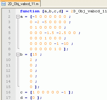
Fig. 1.2.1.3. A file 2D_Obj_vabcd_11.m contents, presented in Notepad ++. Apparently, Vissim has injected all seven state variables (one for an aperiodic link and on two for each oscillating link), but matrixes B and C match to presence in model only the first input and the first output. Matrix D also mirrors presence of one input which has been not linked to outputs
For determination of matrixes b, c and d we will conduct also as well as above, a linearization of the object from each input on each output and we will look at a contents generated by Vissim files:
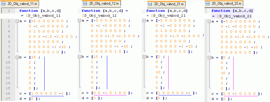
Fig. 1.2.1.4. At each creation of matrixes of state equations Vissim completely determines matrix A, and matrixes of input B and output C are determined only for particular inputs and outputs. Apparently, for obtaining of the complete matrixes B and C it is enough to conduct a linearization only from the first input on the first output and from the second input on the second output
Thus, Vissim at each separate linearization determines all gang of coefficients of a matrix A for all state variables, probably, in the supposition, that further the researcher will connect inputs various modes to this basis, a nucleus and to do outputs.
Having combined manually in the text editor matrix B and C from the first and last files, and also having mirrored that fact, that inputs are not connected up directly, through amplifiers to outputs that gives zero matrix D, of dimensions [2x2] on number of inputs and outputs, we will gain final matrixes of state equations of the control object:
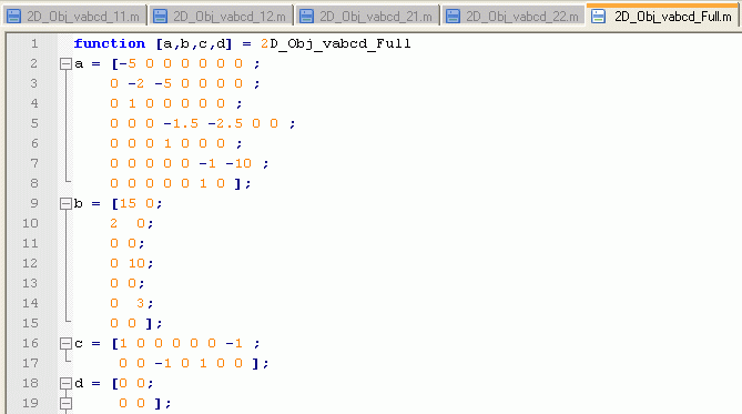
Fig. 1.2.1.5. A set of the complete matrixes of state equations of dynamic 2D-object, a file 2D_Obj_vabcd_Full.m. It is necessary to present matrix D in a view [2 х 2], according to number of object inputs and outputs
How VisSim determines number of state variables and their localisation in the model scheme?
VisSim determines number of integrators in a selection some fragment of scheme , including the integrators disposed in the schemes of submodels. For example, the unit the Transfer function (TransferFunction) the second order has two integrators, the third order - three. State variables concern to outputs of these integrators and consequently their number coincides with number of integrators.
For build-up of the model which are based on state variables, in Vissim it is necessary to carry out on a working field the unit State Space (Blocks - Linear Systems - Statespace). Then, having clicked on the unit the right button, in a dialogue window to indicate a file path with matrixes 2D_Obj_vabcd_Full.m and to click by the button OK. Having given on inputs of the State Space unit trial signals, having attached outputs to the oscilloscope and having started simulation we gain oscillograms which coincide with oscillograms of the initial object, see fig. 1.2.2:
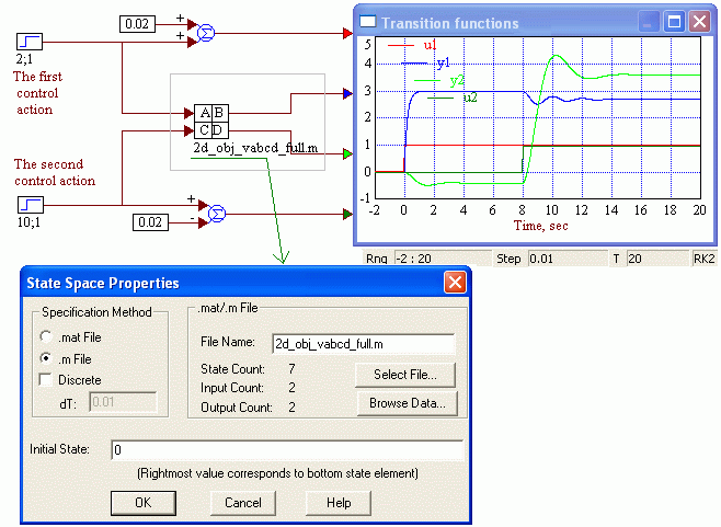
Fig. 1.2.1.6. Simulation of 2D-object by the State Space unit is yielded by the same result, as the initial model made of dynamic links. The model is well-founded. We will mark, that the unit itself, on preset it to a file of matrixes 2D_Obj_vabcd_Full.m determines number of inputs and outputs, representing them on a working fild, and number of state variables, displaying them in a dialogue window at its subsequent opening
Let's uncover partially objective model matching to the StateSpace block fig. 1.2.1.6, having built a dual scheme from separate blocks.
The scheme will be gained enough major, therefore to begin with we will display on working space input of coefficients of matrixes of an input B and an output C:
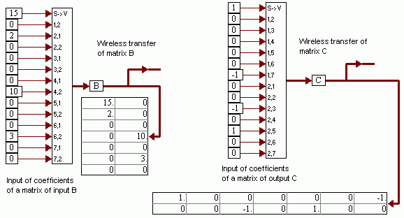
Fig. 1.2.1.7. The input of coefficients of matrixes B and C by means of block ScalarToVec (Blocks - Annotation) transformations of a set of scalars to a vector and wireless transfer of matrixes on their name. Values of coefficients on digital displays appear after simulation activation
Now we will display model of object observed before which is a special case of model fig. 1.2.1.1:
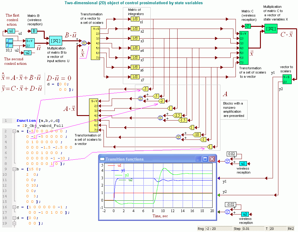
Fig. 1.2.1.8. Vector-matrix model of 2D-object with deployment of matrixes of operators and system matrix A. State equations allow to model the difficult object in a standard vector-matrix kind. Operations of multiplication of a matrix of integrators on a vector of derived state variables, and also multiplication of a matrix A to a vector of state variables are uncovered, displayed in an explicit form for nonzero coefficients of a matrix. Apparently, outcomes of simulation, i.e. model transition functions precisely same, as well as for the initial object builted of assemblage of dynamic units, see fig. 1.2.1.2 and fig. 1.2.1.6
So, matrix B "arranges" with appropriate scales input actions on channels of each state variable. Matrix A returns with appropriate scales state variables to an input of the vector summator, that in the total with weighed by a matrix B input actions gives a vector of derived state variables. This vector is integrated by the matrix integrator, giving values of state variables. The circle was closed.
The gained values of state variables are weighed by a matrix C, giving as a result output variables of the object.
In this case matrix D is zero, also does not pass directly input signals to an output. Therefore appropriate links on model are not displayed not to overcharge the plot.
In a vector-matrix view model in shape fig. 1.2.1.1 will become:
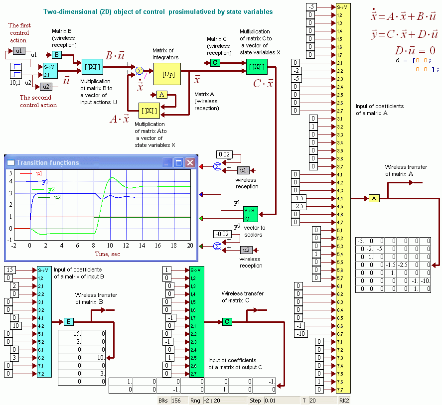
Fig. 1.2.1.9. Representation of model of 2D-object in a matrix form has a compact appearance. Outcomes simulations is the same, as earlier, the model is well-founded. Certainly, the blocks of the input of coefficients of matrixes displayed here for obviousness should be located in the composite block not to overcharge the main working field of model
Model, unlike the real object, allows to look the behaviour of all state variables:
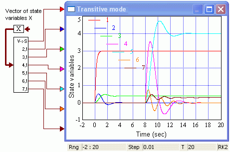
Fig. 1.2.1.10. Oscillograms of state variables of the 2D-object observed above
State variables in case each of them is a derivative on time from previous, are called as phase state variables and in this case they have particular physical sense, as a rule, can be localised and checked in the real object. In some cases state variables can not have at all the is clear enough expressed semantic physical activity, and cannot be localised in the hardware system, and, therefore, and cannot be checked, i.e. are measured. Nevertheless, the object model presented in state variables allows to watch, inspect behaviour of all state variables, fig. 1.2.1.10 see.
Analyzing a matrix of an output C, gained by Vissim it is possible to determine, what output signals of blocks of the initial model builted of dynamic links, match to what state variables:
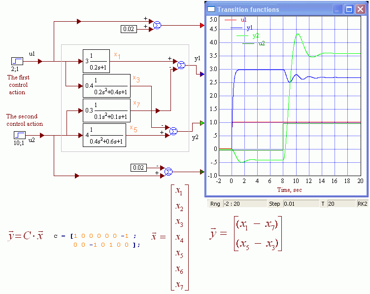
Fig. 1.2.1.11. The matrix of an output C allows to localise state variables in an initial object model. It is simple output signals of appropriate links. Variables х2, х4 and х6 are localised "in" oscillating links
The first variable, apparently on matrix C, is an output signal of an aperiodic link. The seventh variable is an output signal of a link from the second input on the first output. The third variable is an output signal of a link of crossconnection from the first input on second output, and the fifth variable is a link output signal in link of the second input to the second output.
Matrixes of the equations of state variables are necessary to the researcher suffices not so much directly in program Vissim where the model collected from dynamic links, how much can be demanded for the subsequent analytical examination of the object or system and optimisation of its parametres.
Let's mark, that Vissim cannot execute the linearization presented above, with obtaining of matrixes of state equations in the presence of units of delay as a part of an object model. At the analysis of the scheme the branch with a link of delay Vissim simply considers broken. The matter is that in this case at a set of equations of state variables are present not only differential equations, but also algebraic.
Nevertheless, Vissim can be quite used for "automanual" obtaining of matrixes of state equations if in the object there are delay links. It diminishes hand-held routine and labour-consuming operation on conducting of calculations at writing and transformation of system of differential equations of any view to the form of Cauchy, and on forces to any student.
Methods of representation of links of delay at the description of linear objects by state equations, and also writings of the equations with Vissim usage, are observed further.
Other programs, for example PC "MBTY" [4] and Jigrein [5], also allow to determine matrixes of state equations. Moreover, unlike Vissim, these programs have instruments for plotting of frequency characteristics of models with delay links, and, therefore, allow to spend their frequency analysis, in particular to judge a stability degree, i.e. quality of the ARS (automatic regulation system).
In traditional textbooks on a theory of automatic control, for example in [6], by consideration of the description of a linear system in space of state variables usually, most likely, inadvertently, authors hold back that representation of the equations in the classical form of Cauchy allows to present only systems without delay. Certainly, as a rule, the student cannot guess about it, he has enough other problems linked to mastering of a course.
Naturally, exclusion consideration of delay in objects is a method deficiency as essentially narrows down the class of objects which can be analysed a state-variable approach. We will mark, as Vissim is capable to analyse, determine matrixes of the equations of state variables only for models without delay links, see above.
Some rare advanced textbooks, for example [8, the formula (2.1.2)] add a classical set of equations in the form of Cauchy also the auxiliary equations of delay:
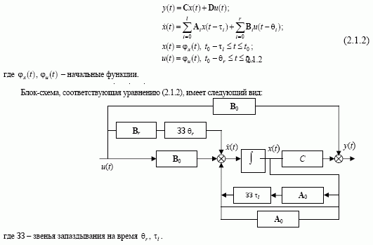
Fig. 1.2.2.1. Consideration of delay in the object by introduction of the auxiliary equations and additional links of delay matching to them [8]
At such description output signals of links of delay do not attribute to state variables. And consequently such representation looks a palliative, the vague solution as the analysis of a conventional matrix of system in which delay links are not considered, for example the stability estimate, loses sense.
Let's consider the multi-dimensional multivariable object, in some or in which all branches there are delay links.
Originally we will describe this object previously having eliminated from it delay links, having substituted their direct hard links. In this case the object without delay can be described in the traditional form of Cauchy (1.2.1.1):
(1.2.2.1)

The first matrix equation in (1.2.2.1) can be recorded in a view
(1.2.2.2)
![]()
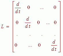
where L - the matrix operator of differentiation:
(1.2.2.3)
Let's return to the complete scheme of the object. Generally, each state variable of the initial model which were not considering delay, can be delayed on some time an appropriate link of delay. Therefore we will add a set of state variables of the equation (1.2.2.2) same number of the state variables matching to output signals of links of delay.
For generalisation of the linear operator of object L (1.2.2.3) it is necessary to inject the formal operator Fwd[x(t), τ], describing the value of function advanced on time its current value on an interval τ:
(1.2.2.4)
![]()
Let's mark, that for the tasks solved in real time, such operator-foreteller, naturally, is not implemented. But for the a posteriori solution [22] when actions are known in advance on all necessary period, for example from a of minus infinite to plus infinite, it is is possible. However, the spent description is routed on obtaining as a result of a structural object model with delay, capable to work in the real time, made on the basis of a state equation. Therefore not too actual problems of the analytical solution of state equations we will leave till the best times.
So, in any branch of an object model there can be a delay link. Moreover, any initial state variable of the object considered without links of delay (1.2.2.2) can retard. We will represent this fact the equation:
(1.2.2.5)
![]()
где LdF – formal matrix operator of differentiation - leading in times:
(1.2.2.6)
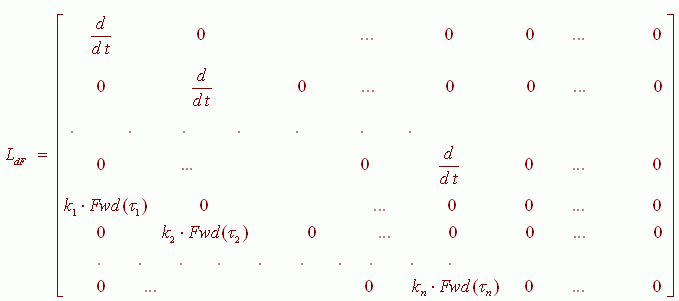
where ki - coefficient, equal to unity if the link of delay for some state variable is available, and it is equal to null if that misses. The maximum dimensions of matrix L dF can be equal to the doubled value of dimensions of matrix L.
Operator matrix LdF is gained from initial operator matrix L by adding of strings of initial state variables matching to time delays. On the right the matrix is added by the same quantity of zero columns.
As can be, not all initial state variables are delayed, that matches ki = 0 these strings and as much zero columns on the right it is eliminated from a final operator matrix.
The matrix of intercommunications between state variables of the object taking into account links of delay will become:
(1.2.2.7)
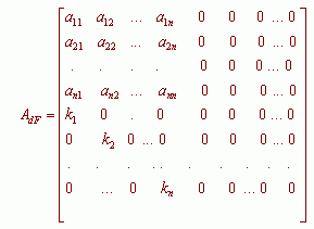
If ki = 0 simultaneously with exclusion of strings and columns in operator matrix LdF it is necessary to make the same and in a matrix of links AdF. In a compact view of matrix LdF and MdF it is possible to present so:
(1.2.2.8)

Matrix AdF as well as earlier, indicates intercommunications between object units. Matrix BdF should contain now as much strings, as matrix LdF and MdF. As to initial "inertia" state variables have been added "retarding" state variables it is necessary to update and the output equation:
(1.2.2.9)
![]()
Matrix CdF contains as much columns, as matrix LdF and MdF, their number is equal to number of state variables.
Let's mark, that the notation of an operator matrix and all other matrixes for methodical reasons is intermediate. The final version of representation is displayed more low.
So, as a result of introduction of the operator of prognosis Fwd, state equations of the object with delay gain the same traditional form:
(1.2.2.10)

However dimensionality of matrixes is increased at number of the state variables matching to links of delay in the object. Besides, the operator matrix along with differentiation operators contains now and operators of prognosis Fwd[x(t), τ].
Essentially, the state equations resulted above, represent all fundamental inertia-dynamic and time-space properties of the continuous linear physical objects, incorporating on both their dynamic properties, and the space expansion of objects and the delay linked to it in propagation of signals and moving of the material bodies. Matrix A determines, mirrors physical links in the object.
The analytical solution of the operator equations (1.2.2.8) does not call special enthusiasm as matrix LdF operator contains operators of the different physical nature: derivations and predictions. At the same time, the structural solution is gained without effort, see more low.
Let's mark also, that the analytical solution allows to estimate the properties of an object model only in an a posteriori regime when actions are known in advance on all timebase [21]. The structural solution, unlike analytical, allows to determine object model response in a real time regime, in process of receipt new, unknown in advance values of actions. In other words, structural, virtual models can work in a real time regime in hardware control systems.
The structural model for the object with delays is under construction by the same principles, as for the object without delay, fig. 1.2.1.1 see. Exterior difference consists only in the denotation and filling up of a matrix of operators.
The matrix of operators of structural models, fig. 1.2.1.1 should be updated by prolongation of a diagonal with integrators by delay operators
(1.2.2.11)
![]()
inverse on operation in relation to the operator of prognosis Fwd, see more low.
Let's display on an instance application of a general concept of state equations for model of the two-dimensional object with delay:
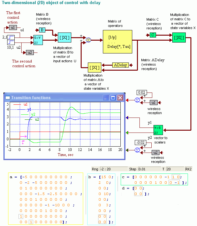
Fig. 1.2.2.2. The 2D-object model in state variables with usage in a matrix of operators not only integrators, but also delay units ensures simulation of objects with delay. Particular values of delay are set in operators of delay of an operator matrix. Matrix A dF is marked out on the scheme for obviousness as ADelay, and in files of Vissim to matrixes titles A, B and C accordingly are saved. Object transition functions precisely same, as well as for the object builted from inertial links with links of delay, see fig. 1.1.2. The model is well-founded. The input of values of coefficients of matrixes A, B and C is spent in the composite block, outside of the working field of Vissim displayed in a figure
The matrix of operators of structural model and particular realisation of this matrix look like this:
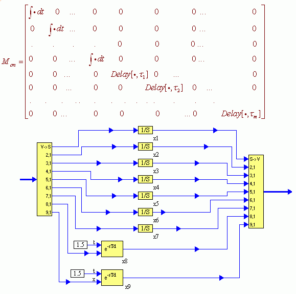
Fig. 1.2.2.2, a. A matrix of operators and contents of the composite block «Matrix of operators»
Modification of an operator matrix and remaining matrixes of a set of state equations was spent manually, on the basis of the analysis of localisation of state variables in an object model with the eliminated links of delay, see fig. 1.2.1.11 and adding of these links of additional state variables matching to output signals.
Senior lecturer SUrSU N.V.Klinachev has offered [14] witty method of localisation of the variables, allowing to detour inability of Vissim to analyse system with delay links: it is necessary to substitute these links by integrators, and then standard tools of Vissim to gain matrixes of state equations. With some addition simplifying localisation of variables, this method looks so:
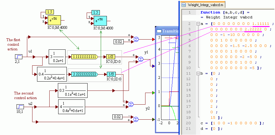
Fig. 1.2.2.3. Substitution of links of delay by integrators and amplifiers with a representative value of gains allow to identify initial model, i.e. to inject and localise the state variables matching to outputs of links of delay. We will mark, that at identification Vissim has added two zero columns in a matrix of links A at the left, instead of on the right as it has been made above. Obviously, these differences do not influence in any way properties of models
Remains, as it has been displayed above, to conduct localisation of state variables, having analysed in Vissim on each pair of inputs and outputs and to update matrixes A, B, C and D.
At last, for reasons of a mathematical aesthetics it is possible to result a matrix A in a view (1.2.2.5) at which the upper left part of a matrix is retracted to "inertia-dynamic" state variables, and lower left - to state variables of links of delay and in appropriate way to update matrixes B and C.
Thus, Vissim allows to "mechanise" process of obtaining of state equations of the object or a control system on their function scheme consisting of links with known transfer functions. It uncloses a path to analytical research of properties of the object as a whole, and also to its simulation by block StateSpace (State variables) in Vissim, and in other programs, for example, PC "MBTY", Jigrein or MVS. It at all does not eliminate necessity of possession of the researcher analytical methods of obtaining of differential equations of the object and their coercion to the generalised form of Cauchy, for example, for validation of obtaining of these equations in simulation programs, but essentially spares a time on execution of transformations.
Modification of an operator matrix and matrixes of state equations , considered above, allows to model objects with delay links in space of state variables.
This modification uncloses a path to the analysis of the complete object model, including to a stability estimate, to a frequency analysis, etc. Problems of an in-depth analysis of objects of delay on their statee quations demand separate consideration. In the given article is put only the modest task to display, that usage of built-in instruments of a simulator, in particular, Vissim, allow to gain at some additional force the equations in state variables for the linear objects of a general view containing not only dynamic links, but also delay links. And it can essentially simplify a life to the student, and the researcher, at obtaining of equations of state, excepting necessity of their obtaining from initial differential equations of the object (the equations of units and links between them).
Let's mark, that inability of Vissim to execute build-up of frequency characteristics of systems with delay it is possible to compensate in a certain methodical procedure [10].
The description of control systems, both linear, and nonlinear, in a state space is much more often uses the mathematicians specialising in a control area, than engineers. Clear matter, representation of the equations in a standard, standard view, allows to develop and apply to the analysis and synthesis of control systems common rigorous and einartig mathematical algorithms. But such description, from the point of view of engineering, not always is optimum.
Really, standard form of state variables equtoins, at all mathematical strictness, not always allows to feel physics, technique of the processes happening in the object, its properties. Generally some state variables can not have at all physical sense and, means, do not allow to feel and adequacy of model to the hardware system or the object, qualitatively to judge a model competence. And optimisation of control systems with usage of a state-variable approach and criteriaa of quality of the automatic control system, for example, minimum root-mean-square error (RMSE), etc., not always leads to excellent results.
Let's mark also:
"To state-space methods the criticism has sounded [3, 18]. In [18] is resulted the instance of the task which are solved in ratio an input-exit and not solved with usage of standard procedures in a state space." [14].
Nevertheless, the state-variable approach at observance of high mathematical accuracy, also can be used at the analysis and synthesis of control systems. Thus it is expedient to apply modified as it is offered above, the form of representation of an operator matrix and system matrixes so that in an explicit form, directly to consider delays in object units.
If there is a real industrial multi-dimensional object of control at build-up of a control system the task of its identification originates, i.e. build-ups of its some mathematical model. One of kinds of such models, the type model «Input - Output» is. It is simple in understanding, is evident, directly mirrors effect of each input value on the output.
For obtaining of the linear object model of control of type «Input - Output» is enough to conduct determination of transition curves of the object on each input, determining transition curves on each output:
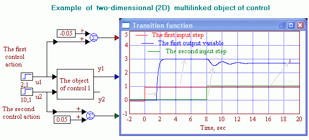
Fig. 1.2.3.1. Transition functions on the first output of the identified object of control on the first and second inputs
On transition functions in a considered instance it is easy to determine, that on the channel «the first input - the first output» link incorporates in-series an aperiodic link, with an amplification 3 and time constant of 0.2 sec, and a delay link on 1.5 seconds. The link from the second input on the first output has an amplification 0.3, this oscillating link with parametres which can be determined on character of a transition function, and its output signal is summed up with an output signal of a feedforward 1 - 1 with the subzero sign.
Let's mark, that frequently the control object is nonlinear. Therefore its linear model can be gained, having established nominal of input values, i.e. control and disturbing actions, and their graduated gains should be made small in comparison with nominal values. As a result the object linearization in its nominal regime will be executed and under oscillograms the structure of models of its branches is gained.
The analysis of the complete nonlinear model is more difficult. But it is possible to reduce it to the previous case, sequentially adding in input graduated actions direct components, and then changing them [19, 20]. A principle of an illustration of identification of the nonlinear object which was offered in personal contact with the author in May, 2009 by the senior lecturer of the Euroasian national university of Gumilev (Kazakstan), k.t.s. (phd) Kulmamirov S.A. can present the animation made in Mathcad:
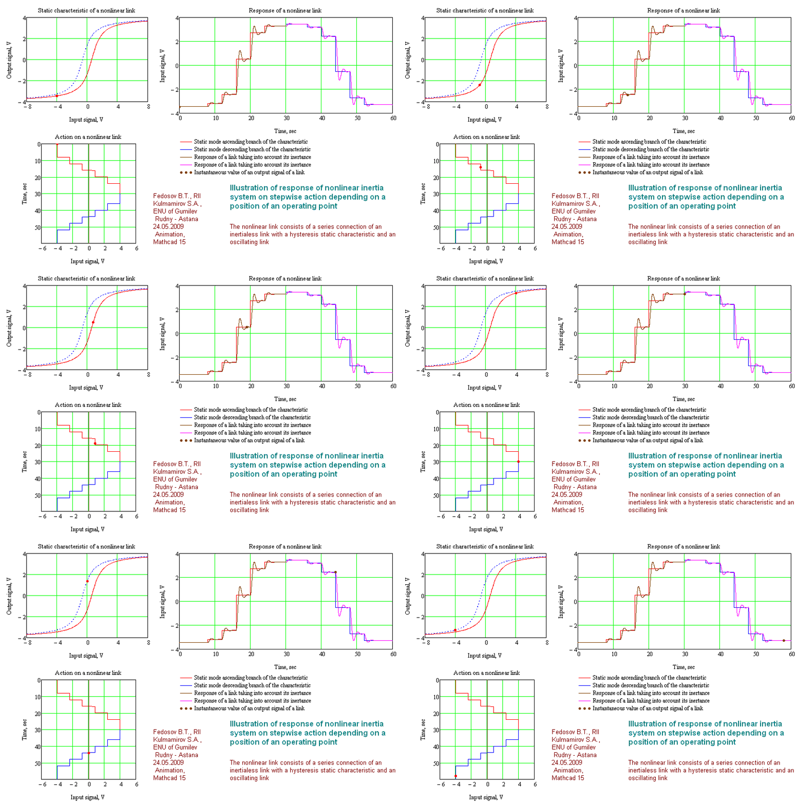
Fig. 1.2.3.2. (Animation, 36 frames). An illustration of a method of autodetection of a static characteristic and differential dynamic properties of the one-dimensional nonlinear inertia object
There is also an assemblage of other methods of identification of real objects [11; 18, Item 1; 19, item 3.3].
There is nothing good if at adding of gas the car starts to turn together with a speed-up to the right, and at decrease of supply of gas to decrease speed, but to turn on the left. Such interaction interference of controlling variables on some operated in practice try to eliminate, i.e. to save effect of each controled variables on one, the "own" operated. Or, at least control actions so to divide into groups that one controlled variable submitted to each group only.
The isolation of actions can be executed by automatic control systems, both open-loop and closed-loop automatic regulation system
The open ARSes (automatic regulation systems) with control on disturbance are stable, but not so accurate and have rather a fast response time. Happens difficultly to consider, gauge and compensate all factors leading to tracking errors. Rather low accuracy of the open ARS (automatic regulation system) with control on disturbance is linked with it, in particular.
At control of multi-dimensional objects by means of closed ARSes (automatic regulation systems) parallel control, or if it is is possible, control on the basis of the subordinate regulating with division of enclosure contours on fast operation when the ARS (automatic regulation system) reminds a matrioshka is applied: the "fast" interior control loop is embraced exterior, sluggisher. As "another's" actions are disturbances at an ARS (automatic regulation system) parallel operation their assemblage structure for the ARS (automatic regulation system) of some controlled variable so that their fast operation was essentially discriminated. Then "fast" auxiliary ARSes (automatic regulation systems) will have time to ensure requirements of correct functioning of the ARS (automatic regulation system) of a principal controlled variable.
As effect on some controlled variable of the object «not own» actions can be considered the as disturbance, principle Chikolev - Poncelet, a principle of control on disturbance, can be applied to it more or less complete compensation, i.e. stabilising of some output controlled variable of the object by action on a principal control channel a signal opposite to disturbance. The compensation factor is determined by an exactitude of determination of variable of disturbance and instability of gains of crossconnections of the object.
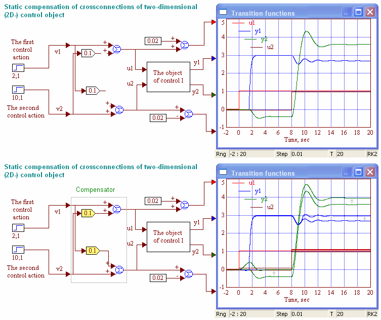
Fig. 2.1.1. (Animation, 2 frames). Adding to each input action a part second with an opposite sign it is possible to eliminate a considerable proportion of cross effects in a statics. Dynamics compensation (inertances and oscillatorility) and delays by control on disturbance is not realizable, as the transfer function of the compensatory arrangement should be return in relation to a transfer function of appropriate crossconnection that leads to a not implemented link
Known deficiency of control on disturbance in the open ARS (automatic regulation system) is the zero information for the regulator about real deviation of a controlled variable from a desired value. It is disadvantage of open-circuit systems which does not allow to execute compensation of effect of factors not considered in model. Advantage of the open ARS (automatic regulation system) - stability and rather high, in relation to systems with control on deviation, fast operation.
It is useful to consider and the solution of a specific task on an elimination of a cross interferences of control actions and disturbances in system with control on disturbance in a static regime.
More often in the important control systems is applied high-precision control on deviation which guesses feed-back loop presence. The contour (loop), on the one hand, allows the regulator to be well informed about what at present a controlled variable and accordingly to adjust a controlling variable. But, on the other hand, contour (loop) presence creates also potential danger losses of stability by it.
The singularity of multi-dimensional objects with cross effect of actions on controlled variables at control of them on deviation consists in origination of the additional loops which are containing crossconnections which also can lose stability at an unsuccessful combination of parametres and structures of ARS (automatic regulation system).
Let's consider some exemples.
Let each controlled variable of the two-dimensional object is operated by it's own contour. Crossconnections, adding links straight lines, organise also an additional, third contour, in the form of "figure of eight":
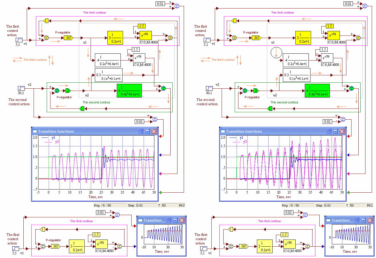
Fig. 2.2.1 (animation, 2 frames). The multivariable object has some contours, each of which potentially can be unstablis. In this case the first contour only is unstablis, moreover, the third contour which is looking like "figure of eight", plays though also insignificant, but a stabilising role as at a breaking of link 1-2 third contours (a frame 2 of animations) the velocity of increment of amplitudes of output signals is increased
Control on deviation ensures not only tracing, but also, indirectly, stabilising, i.e. compensation of cross effect of disturbances, however systems of control on deviation potentially are unstablis. Optimising gains P-regulators, we will gain:
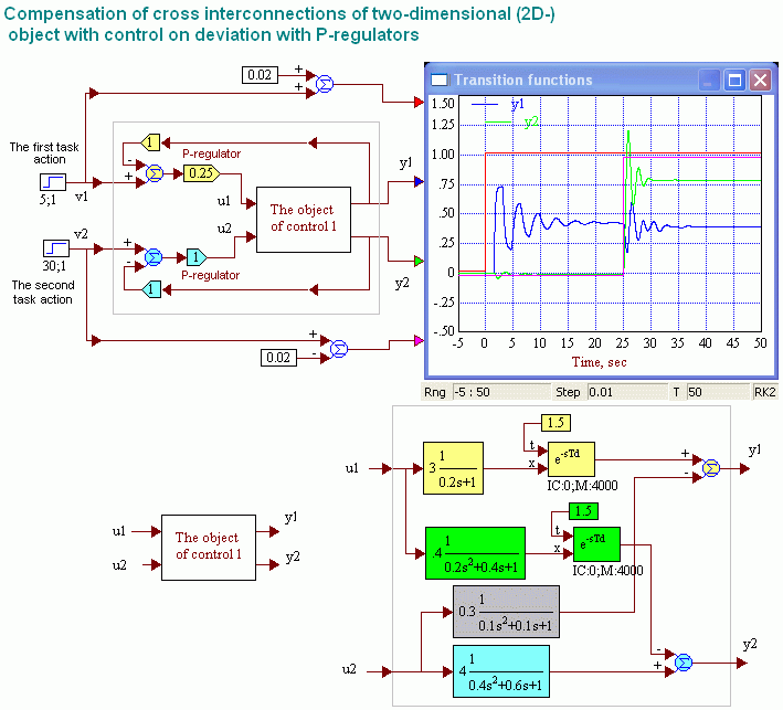
Fig. 2.2.2. The ARS (automatic regulation system) with control on deviation with P-regulators on each channel has two feedback. The ARS is stable, but has rather poor quality of regulating. Crossconnections in the control object lead to that each action influences each controlled variable. Apparently, in the given instance effect of the second action on first is much stronger, than first on the second. The ARS (automatic regulation system) with P-regulators does not manage tracing as in a transient regime: there is a heightened oscillatorility, and in the established: errors are very great, on the first channel it is 60 %, on the second 20 %. Magnification of an amplification of P-regulators will lead to loss of stability by system, decrease - to a decline and without that to an unsatisfactory accuracy of regulating. All it is stipulated by presence of a link of delay with rather long delay in the first forward channel
PI-regulators quite manages to control in the ARS (automatic regulation system) with the considered two-dimensional multivariable object:
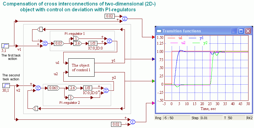
Fig. 2.2.3. The optimum PI-regulators located in control loops on each controlled variable, ensure high quality of tracing and stabilising (compensation of cross effect of actions). Transient response time is determined by a delay factor in links of delay of the object
Let's mark, that tuning of regulators can be conducted in Vissim and in an automode. Principles and instances of self-acting optimisation on a number of criteriaa of quality are considered in details in [17].
Thus, at control of multi-dimensional objects it is necessary to consider and a capability of origination of instability in contours, organised by crossconnections and to eliminate it.
... See the complete version (russian)
The Drying aggregate as an educational exemple is selected because the principle of its operation is obvious and pellucid, that allows to concentrate on the main task of the present article - build-up and learning of a multi-dimensional object model of control.
... See the complete version (russian)
Multi-dimensional objects are described in dynamics by a matrix of the transfer functions linking the Laplace image of a signal on each output of the object with the Laplace image on each input. The object matrix contains in a statics simply the numerical coefficients indicating, what amplification on what channel has the object. This description on a method «Input - Output».
Other method of the description is the description by the state equations using state variables. Advantage of this method that they can describe and analyze both linear, and nonlinear objects and control systems.
Program Vissim allows to simplify, automize obtaining process as matrixes of the equations «Input - utput», and matrixes of state equations.
At control of multi-dimensional objects their crossconnections potentially can lead to loss of ARS (automatic regulation system) stability.
Operator integration - delays the M оп is the matrix operator representing a scalar matrix which units of a diagonal are operators of integration and (or) delay operators. This operator uses in models of objects and the control systems described by state equations.
The State variable object models it is the mathematical variable varying in time which are a numerical index of its some characteristic both in an autonomous mode of functioning, and at external actions. The instantaneous value of assemblage of state variables completely characterises a status of model of the inertia object, and the change of assemblage of state variables in time completely characterises behaviour of the object. Output variables of the linear object of control are a linear combination of state variables. If each state variable is a derivative on time from a state variable with previous number such variables name the phase variables.
The State equations it is two matrix equations, i.e. assemblage of two linear systems of the equations. The first system consists of a standard kind of linear differential equations and describes both interior dynamic properties of the object, and effect of external actions on its state variables. The second set of equations links output variables of the object to its state variables, and also, can be and with other actions (input control values or noise, the reasons of measurement errors of output variables, etc.).
Remarks. The significant number of determinations of the concepts linked to control by objects is given in [22].
The author expresses gratitude to senior lecturer of SUSU (Chelyabinsk), c.t.s. (Phd) Klinachev N.V. for the useful discussion of problems of the description and the analysis of multi-dimensional objects.
Rudny, Kazakhstan. 17.07.2010 - 8.08.2011